Sky Map of Milky Way

Introduction

MWSkyMap class is a wrapper around the matplotlib library to plot the sky map of the Milky Way. It provides a simple interface to plot the sky map with different projections, background images, and grid lines. The class is designed to be simple and easy to use.

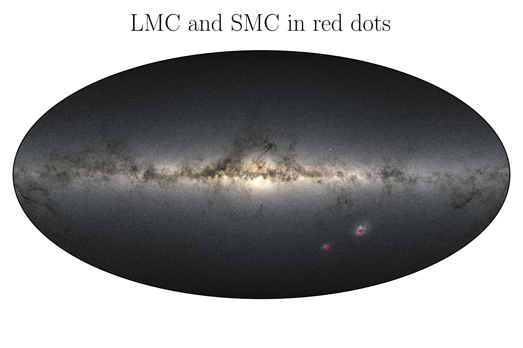
>>> from astropy import units as u
>>> from mw_plot import MWSkyMap

>>> mw1 = MWSkyMap(projection="aitoff", grayscale=False)
>>> mw1.title = "LMC and SMC in red dots"
>>> mw1.scatter([78.77, 16.26] * u.degree, [-69.01, -72.42] * u.degree, c="r", s=3)

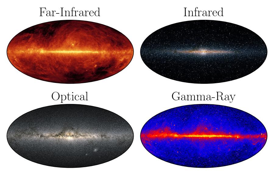
Background Images

mw_plot use Gaia DR3 as the default background image. But a few background images are included within the package which represent optical, gamma, far-infrared and infrared such that they can be used even without an internet connection to fetch images.

For other background images from Hierarchical Progressive Surveys (HiPS), you can use the search_sky_background method to search for available HiPS images. HiPS of the code has made use of the hips2fits, a tool developed at CDS, Strasbourg, France aiming at extracting FITS images from HiPS sky maps with respect to a WCS.

You can search for list of available HiPS images with keywords by using the following code

You can search for HiPS images with specific keywords. For example

>>> from mw_plot import MWSkyMap
>>> MWSkyMap.search_sky_background(keywords="extragalactic optical color")
['Mellinger color optical survey']

will return a list of all available HiPS images came from Gaia DR3. If no keyword is given (i.e. None), the function will return a list of all available HiPS images.

You then can use the background parameter to set the background image from the search result. For example

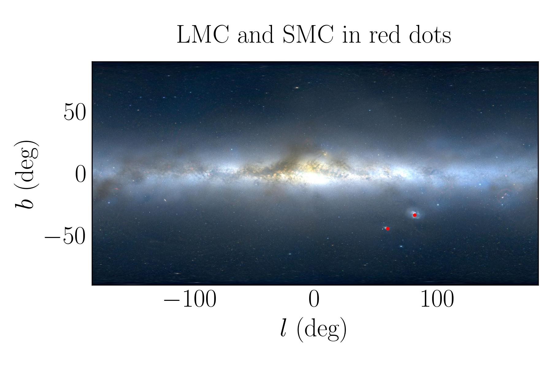
>>> from astropy import units as u
>>> from mw_plot import MWSkyMap
>>> mw1 = MWSkyMap(background="Mellinger color optical survey")
>>> mw1.title = "LMC and SMC in red dots"
>>> mw1.scatter([78.77, 16.26] * u.degree, [-69.01, -72.42] * u.degree, c="r", s=3)

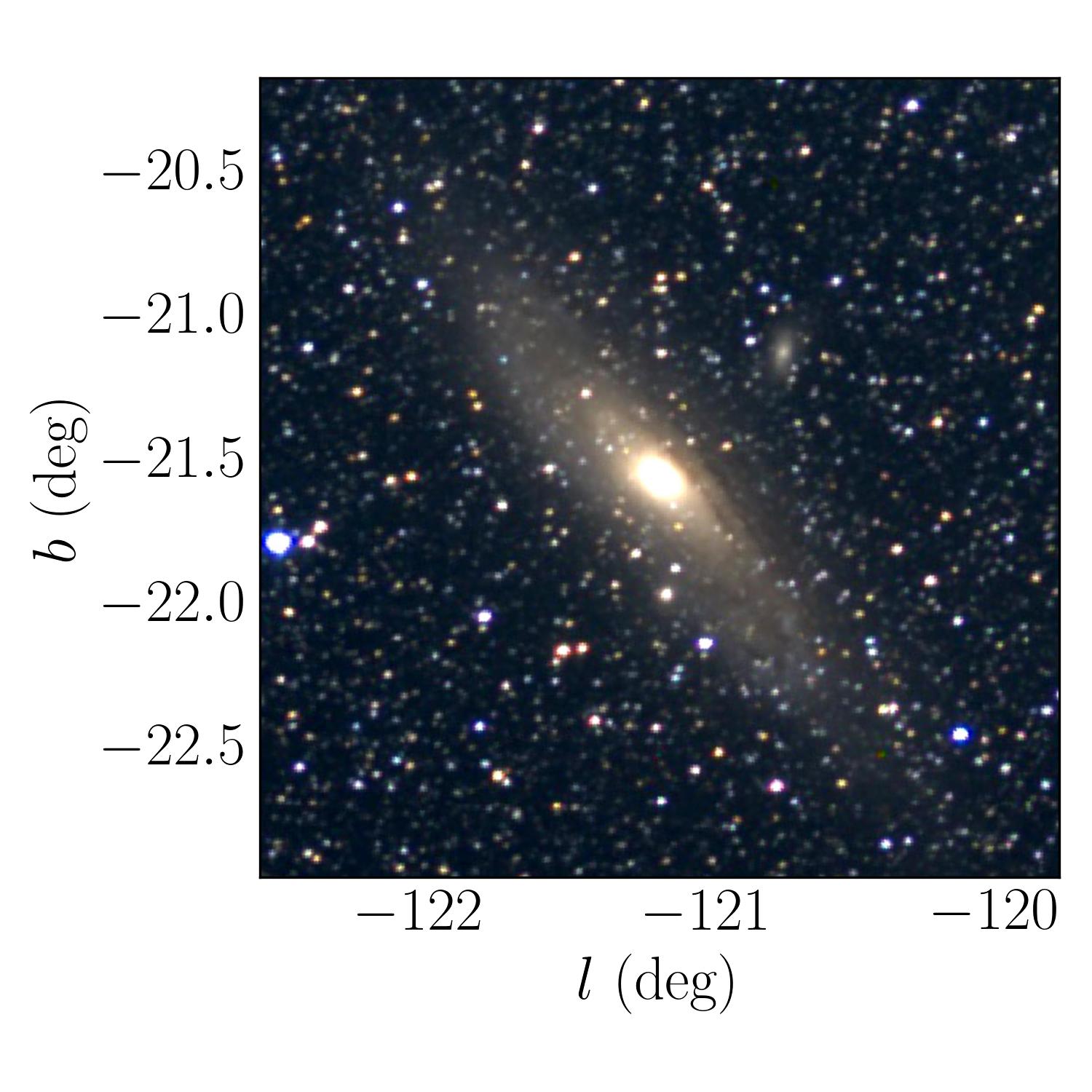
You can also zoom in to a specific region of the sky by setting the center and radius parameters. For example to zoom in to the M31 galaxy, you can use the following code

>>> import matplotlib.pyplot as plt
>>> from astropy import units as u
>>> from mw_plot import MWSkyMap
>>> mw1 = MWSkyMap(
...     center="M31",
...     radius=(4000, 4000) * u.arcsec,
...     background="Mellinger color optical survey",
... )
>>> fig, ax = plt.subplots(figsize=(5, 5))
>>> mw1.transform(ax)

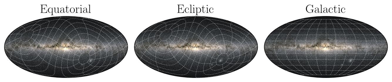
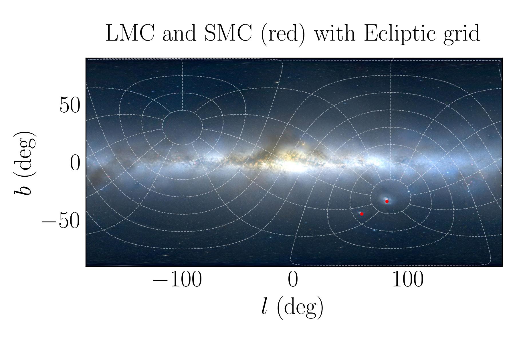
Celestial Grids

You can plot the sky map with grid lines. The grid lines can be in Galactic, Equatorial, or Ecliptic coordinates.

>>> from astropy import units as u
>>> from mw_plot import MWSkyMap
>>> mw1 = MWSkyMap(background="Mellinger color optical survey", grid="ecliptic")
>>> mw1.title = "LMC and SMC (red) with Ecliptic grid"
>>> mw1.scatter([78.77, 16.26] * u.degree, [-69.01, -72.42] * u.degree, c="r", s=3)

Class API

class mw_plot.MWSkyMap(grayscale: bool = False, projection: str = 'equirectangular', background: str = 'optical', center: ~typing.Tuple[float, float] | str = <Quantity [0., 0.] deg>, radius: tuple = <Quantity [180., 90.] deg>, grid: str = None, figsize: ~typing.Tuple[float, float] = (6, 4))

MWSkyMap class plotting with Matplotlib

Parameters

grayscalebool, optional

Whether to use grayscale background. The default is False.

projectionstr, optional

Projection of the plot. The default is “equirectangular”.

backgroundstr, optional

Background image of the plot. The default is “optical”. You can use MWSkyMap.search_background(keyword=None) to search for available background images.

centerUnion[Tuple[float, float], str], optional

Center of the plot. The default is (0.0, 0.0) * u.deg.

radiustuple, optional

Radius of the plot. The default is (180.0, 90.0).

gridstr, optional

Grid of the plot. The default is None.

figsizeTuple[float, float], optional

Matplotlib figure size. The default is (5, 5).

annotate(*args, **kwargs)

Plot annotation

History:

2022-Jan-02 - Written - Henry Leung (University of Toronto)

initialize_mwplot(fig=None, ax=None, _multi=False)

Initial mw_plot images and plot

Returns:

None

mw_scatter(ra, dec, c='r', **kwargs)

Plot scatter points with colorbar

Parameters:

• ra (astropy.Quantity) – Scatter points x-coordinates on the plot

• dec (astropy.Quantity) – Scatter points y-coordinates on the plot

• c (Union[str, list, ndarry]) – Scatter points color

History:

2018-Mar-17 - Written - Henry Leung (University of Toronto)

scatter_annotate(text, position, arrowprops={'facecolor': 'black', 'headlength': 6.0, 'headwidth': 6.0, 'width': 1.0}, fontsize=15, bbox={'pad': 2}, **kwargs)

Plot annotation with scatter

History:

2022-Jan-02 - Written - Henry Leung (University of Toronto)

transform(x)

Transform matplotlib figure or a single axes